Python Basics #4: Pandas

This is post four in our series Python Basics, where we discuss the minimum Python and Jupyter you need to know to successfully automate Excel reports using Mito. Read Post One: Hello World, Post Two: Variables, and Post Three: Functions.

So far, we've used variables to hold individual values, for example the string "Hello World". But since our goal is to migrate an entire Excel report to Python, we need a way of working with entire tables of data.

The pandas Python package was developed exactly for that – making it easy to analyze data that is organized in rows and columns.

You can think of Python packages like this: In Excel, there is built-in functionality that allows you to manipulate your data. Things like sorting and filtering. But you can also install plugins that give you new functionality above and beyond what is built into Excel. That's exactly how Python packages work. A package is a set of functions that you can import into your code to perform specific tasks. The pandas package, for example, contains functions for working with tabular data.

The pandas package gives you this additional functionality through a special kind of variable called a pandas dataframe. Think of a Pandas dataframe as an entire sheet in Excel – it has rows and columns of data, and each column has a name. We call each column a series.

Transforming data in a dataframe

In pandas, you can manipulate the data in a dataframe using a variety of functions, just like you would in a spreadsheet. For example, you can sort, filter, and pivot your data.

Manipulating your data in Excel is easy. Manipulating your data in pandas is a bit more challenging -- that's why Mito exists. Mito makes writing pandas code as easy as using Excel. Notice in the video below that whenever we edit our data in the Mito spreadsheet, the equivalent Python and pandas code is generated in the code cell below.

Let's take a look at the code that Mito generated to understand what's going on.

In line 1, we're importing the pandas python package so we can use its functionality in our script.

In line 4, we're using the pandas function read_csv to read the file named loans.csv and turn it into a pandas dataframe called loans. In other words, we've created a variable called loans that contains our tabular data.

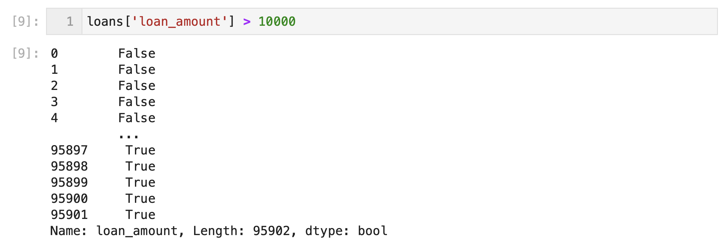
In line 7, we're filtering our dataframe to only display rows that have a value in the loan_amount column greater than 10,000. Let's take a closer look at this line of code – there are a few important concepts to unpack.

• loans['loan_amount']: This selects the loan_amount column from the dataframe named loans. Whenever we want to access a specific column in pandas, we use this syntax.
• loans['loan_amount'] > 10000: The output of this line is a series of True/False values, where True indicates that the loan_amount is greater than 10,000 and False indicates that it is not. If we just ran this subset of the code, we'd generate the series below. Notice that for every row in our loans dataframe, there is a True or False label.

• loans[loans['loan_amount'] > 10000]: This applies the True/False series to the loans dataframe to select only the rows where the loan_amount is greater than 10,000.
• loans = loans[loans['loan_amount'] > 10000]: This updates our loans variable to represent the new dataframe that has all of the rows with a loan_amount less than 10,000 filtered out.

So, the overall effect of this code is to create a new DataFrame called 'loans' that contains only the rows where the loan_amount is greater than 10,000.

Stay tuned for the next post in this series where we'll learn how to turn the pandas code that Mito generates into a function so we can apply it to multiple dataframes.